Electricity and physics lessons - Bastion Circuit Designer manual

A comprehensive engineering handbook and pedagogical physics curriculum integrated directly into the Bastion EDA environment.

Open-Source Curatorial References & Pedagogical Foundations

This curriculum and Bastion's built-in Physics & Electricity Academy (Ctrl+Shift+L) are written in-house and cite the free, commercially reusable references listed below (public domain, CC0, CC BY, or CC BY-SA when the source is only linked and never copied):

Tony R. Kuphaldt — Lessons In Electric Circuits (Vol. I DC, Vol. II AC, Vol. III Semiconductors, Vol. IV Digital) under the Design Science License (DSL).
Public-domain classics — A. P. Morgan, The Boy Electrician (Project Gutenberg ebook 63207); Maxwell, A Treatise on Electricity and Magnetism (1881); Steinmetz, Theory and Calculation of Alternating Current Phenomena (1897).
Wikipedia — encyclopaedia articles, linked as pointers only (CC BY-SA 4.0), whose text is never copied.
Vendor datasheets and public standards — the device and interface references named inside each lesson.

Curriculum Structure & Table of Contents

| #| Topic| Category| Governing Physical Law| Primary Formula| Associated Components| | 1| Voltage & Electromotive Force| Fundamentals| Electric Potential Definition| \(V = \frac{W}{Q}\)| Voltage Sources, Batteries, VCC Rail| | 2| Current & Charge Drift Velocity| Fundamentals| Charge Conservation / Amperage| \(I = \frac{dQ}{dt} = n q A v_d\)| Ammeters, Series Loops| | 3| Circuit Ground & Reference Potential| Fundamentals| Gauss's Law / Earth Equipotential| \(V_{\text{GND}} = 0.0\text{ V}\)| Ground (GND), Earth, Chassis| | 4| Ohm's Law & Joule Heating| Fundamentals| Constitutive Resistive Relation| \(V = I \cdot R,\; P = I^2 R\)| Resistors, Trimpots, Heaters| | 5| Voltage Dividers & Thevenin Equivalence| Analysis| Conservation of Energy & Linearity| \(V_{\text{out}} = V_{\text{in}} \cdot \frac{R_2}{R_1 + R_2}\)| Potentiometers, Dividers| | 6| Capacitance, Dielectrics & RC Transients| Passives| Maxwell-Gauss / Displacement| \(i_C(t) = C \frac{dv}{dt},\; \tau = R C\)| Ceramic, Electrolytic Capacitors| | 7| Inductance, Faraday's Law & Back-EMF| Passives| Faraday-Lenz Electromagnetic Induction| \(v_L(t) = L \frac{di}{dt}\)| Inductors, Chokes, Flyback Coils| | 8| P-N Junctions & Diode Rectification| Semiconductors| Shockley Ideal Diode Equation| \(I_D = I_S \left(e^{\frac{V_D}{n V_T}} - 1\right)\)| 1N4148, 1N4007, Rectifiers| | 9| Light Emitting Diodes & Optoelectronics| Semiconductors| Planck-Einstein Photoelectric Relation| \(E_g = \frac{h c}{\lambda},\; R_{\text{lim}} = \frac{V_S - V_F}{I_F}\)| LEDs, Optocouplers| | 10| Zener Breakdown & Voltage Regulation| Semiconductors| Quantum Zener Tunneling & Avalanche| \(V_Z = \text{const}\) (for \(I_Z \ge I_{ZK}\))| Zener Diodes, Clamps| | 11| Transistors: BJT Current & MOSFET Field| Semiconductors| Ebers-Moll & MOSFET Saturation| \(I_C = \beta I_B,\; I_D = \frac{1}{2} k_n' \frac{W}{L} (V_{GS} - V_{th})^2\)| 2N3904 (NPN), 2N3906 (PNP), MOSFETs| | 12| Operational Amplifiers & Golden Rules| ICs & Analogs| Negative Feedback Virtual Short| \(V_+ = V_-,\; I_+ = I_- = 0\)| LM358, TL072, Op-Amps| | 13| The 555 Timer IC & Multivibrator Dynamics| ICs & Analogs| RC Threshold / Trigger Flip-Flop| \(f = \frac{1.44}{(R_1 + 2R_2)C}\)| NE555 Timer| | 14| Boolean Logic & CMOS Gates| Digital Logic| Switching Algebra & CMOS Pull-up/down| \(Y = \overline{A \cdot B},\; \overline{A + B}\)| 74HC00, 74HC08, 74HC04| | 15| Microcontrollers & GPIO Interfacing| Digital Logic| CMOS Input/Output Driver Limits| \(I_{\text{GPIO}} \le 20\text{ mA},\; V_{IH} \ge 0.7 V_{CC}\)| ESP32, ATmega328P, RP2040| | 16| Oscilloscopes & Time-Domain Metrology| Instruments| Nyquist-Shannon Sampling Theorem| \(f_{\text{sample}} \ge 2 f_{\text{max}},\; BW \ge 5 f_{\text{signal}}\)| Virtual Scope, Probes| | 17| Multimeters & Shunt Measurement| Instruments| Galvanometer D'Arsonval & Burden Voltage| \(I = \frac{V_{\text{shunt}}}{R_{\text{shunt}}},\; R_{\text{in}} \ge 10\text{ M}\Omega\)| Virtual DMM, Voltmeter| | 18| Kirchhoff's Laws (KCL & KVL)| Analysis| Conservation of Charge & Energy| \(\sum I_{\text{node}} = 0,\; \sum V_{\text{loop}} = 0\)| Wires, Nets, Junctions|

In-Depth Lesson Modules

Module 1: Voltage & Potential Difference

Open-Source Attribution: Kuphaldt, Vol I, Chapter 1.
Physical Concept: Electrostatic potential difference is the work required per unit charge to move a test charge between two points against an electrostatic field: \(V_{AB} = -\int_A^B \vec{E} \cdot d\vec{\ell}\) In lumped circuit theory, potential difference is measured in Volts (\(1\text{ V} = 1\text{ J}/\text{C}\)). It acts as the electrical "pressure" that induces drift current through conductive pathways.
Governing Equations: \(V = \frac{W}{Q},\quad \vec{E} = -\vec{\nabla} V\)
Engineering Rule of Thumb: Always decouple DC power rails with a \(100\text{ nF}\) ceramic capacitor placed immediately adjacent to every IC's \(V_{CC}\) pin to absorb transient high-frequency voltage sag caused by trace inductance.

Module 2: Electric Current & Charge Drift Velocity

Open-Source Attribution: Kuphaldt, Vol I, Chapter 2, Chapter 9.
Physical Concept: Electric current is the net macroscopic rate of electrical charge transport through a cross-sectional area: \(I = \frac{dQ}{dt}\) Although individual conduction electrons drift remarkably slowly (drift velocity \(v_d \approx 10^{-4}\text{ m/s}\) in copper under typical fields), the electromagnetic wavefront propagates through the dielectric medium surrounding the conductor at approximately \(0.6c\) to \(0.7c\) (\(\sim 200{,}000\text{ km/s}\)).
Governing Equations: \(I = n \cdot q \cdot A \cdot v_d,\quad J = \sigma E = \frac{I}{A}\)
Engineering Rule of Thumb: For standard \(1\text{ oz/ft}^2\) (\(35\text{ }\mu\text{m}\)) copper PCB traces, budget approximately \(1\text{ mm}\) trace width per \(1\text{ A}\) of continuous direct current to maintain a trace temperature rise under \(10^\circ\text{C}\).

Module 3: Circuit Ground & Reference Equipotentials

Open-Source Attribution: Kuphaldt, Vol I, Chapter 3; Henry Ott, Electromagnetic Compatibility Engineering.
Physical Concept: Voltage is an inherently relative scalar quantity: voltage exists only between two spatial coordinates. "Ground" (GND) is an arbitrary but vital reference node designated by convention as \(0.0\text{ V}\). In high-frequency and low-noise electronics, ground is not a zero-impedance sink, but a return path through which all currents loop back to their energy sources.
Governing Equations: \(V_{\text{node}} = V_{\text{node}} - V_{\text{GND}},\quad Z_{\text{return}} = R_{\text{dc}} + j \omega L_{\text{loop}}\)
Engineering Rule of Thumb: Avoid ground loops. High-frequency return currents travel directly underneath the signal trace on the nearest continuous ground plane to minimize loop inductance (\(L_{\text{loop}}\)). Never split ground planes underneath fast digital or analog signal lines.

Module 4: Ohm's Law & Joule Heating

Open-Source Attribution: Kuphaldt, Vol I, Chapter 2, Chapter 9.
Physical Concept: Ohm's Law describes the linear relationship between the electromotive potential drop across an ohmic conductor and the resulting current. Collisions between accelerated electrons and the metallic crystal lattice convert electric potential energy irreversibly into thermal kinetic energy (Joule heating).
Governing Equations: \(V = I \cdot R,\quad P = V \cdot I = I^2 R = \frac{V^2}{R}\)
Engineering Rule of Thumb: Never operate carbon film or SMD thick-film resistors at greater than \(50\%\) to \(60\%\) of their continuous rated power dissipation (e.g., limit a \(0.25\text{ W}\) 0805 resistor to \(\le 0.125\text{ W}\)) to ensure low thermal drift and prevent premature aging.

Module 5: Voltage Dividers & Thevenin Equivalence

Open-Source Attribution: Kuphaldt, Vol I, Chapter 6 & 10.
Physical Concept: Two series resistors divide an input voltage in direct proportion to their resistances. However, connecting any finite load resistance \(R_L\) in parallel with \(R_2\) draws current and reduces the effective output voltage (loading effect). Thevenin's theorem models any linear two-terminal resistive network as a single ideal voltage source \(V_{th}\) in series with an equivalent resistance \(R_{th}\).
Governing Equations: \(V_{\text{out}} = V_{\text{in}} \cdot \frac{R_2}{R_1 + R_2},\quad R_{th} = R_1 \parallel R_2 = \frac{R_1 \cdot R_2}{R_1 + R_2}\)
Engineering Rule of Thumb: To prevent noticeable loading errors (\(<1\%\)), design voltage divider bleeders such that the divider resistance \(R_2\) is at least \(10\times\) to \(100\times\) smaller than the load impedance \(R_L\), or buffer the output with a unity-gain op-amp follower.

Module 6: Capacitors, Dielectrics & RC Transients

Open-Source Attribution: Kuphaldt, Vol I, Chapter 13, Chapter 8.
Physical Concept: A capacitor stores electrostatic potential energy within the polarized electric field of its dielectric material. The instantaneous current through a capacitor is proportional to the time rate-of-change of voltage (\(i = C \frac{dv}{dt}\)). Consequently, the voltage across a capacitor cannot change instantaneously.
Governing Equations: \(Q = C \cdot V,\quad i_C(t) = C \frac{dv}{dt},\quad v_C(t) = V_{\text{final}} + (V_{\text{initial}} - V_{\text{final}}) e^{-t / \tau},\quad \tau = R \cdot C\)
Engineering Rule of Thumb: An RC transient circuit reaches \(63.2\%\) of its target step voltage in \(1\tau\), and effectively completes its charge/discharge cycle (\(>99.3\%\)) after \(5\tau\). For power decoupling, place low-ESR ceramic caps (\(0.1\text{ }\mu\text{F}\)) as close as physically possible to IC pins.

Module 7: Inductance, Faraday's Law & Back-EMF

Open-Source Attribution: Kuphaldt, Vol I, Chapter 14, Chapters 13-14.
Physical Concept: Inductance is the property of an electric circuit that opposes any instantaneous change in current. By Faraday's Law of Induction and Lenz's Law, when current through an inductor collapses rapidly (\(\frac{di}{dt} \ll 0\)), the collapsing magnetic field induces an electromotive force (Back-EMF) that opposes the change, generating massive voltage spikes.
Governing Equations: \(v_L(t) = L \frac{di}{dt},\quad E_{\text{stored}} = \frac{1}{2} L I^2,\quad f_0 = \frac{1}{2\pi \sqrt{L C}}\)
Engineering Rule of Thumb: Always connect a reverse-biased flyback diode (such as a 1N4007 or Schottky diode) in antiparallel across inductive coils, relays, solenoids, and DC motors to clamp inductive kickback spikes and protect switching transistors from avalanche breakdown.

Module 8: P-N Junctions & Diode Rectification

Open-Source Attribution: Kuphaldt, Vol III (Semiconductors), Chapter 2; Streetman & Banerjee, Solid State Electronic Devices.
Physical Concept: The interface between p-type and n-type semiconductor regions forms a depletion layer devoid of free charge carriers. Under forward bias (\(V_D > V_F \approx 0.7\text{ V}\) for Silicon), the internal potential barrier is overcome, permitting exponential majority carrier diffusion. Reverse bias widens the barrier, restricting current to microscopic reverse saturation current \(I_S\).
Governing Equations: \(I_D = I_S \left(e^{\frac{q V_D}{n k_B T}} - 1\right) = I_S \left(e^{\frac{V_D}{n V_T}} - 1\right)\) (At room temperature \(T = 300\text{ K}\), thermal voltage \(V_T \approx 25.85\text{ mV}\)).
Engineering Rule of Thumb: Silicon diodes exhibit a nominal \(0.65\text{ V}\) to \(0.7\text{ V}\) forward drop at moderate currents. For high-efficiency or low-voltage solar/battery circuits, use Schottky barrier diodes (e.g. 1N5819) which feature a forward drop of only \(0.2\text{ V}\) to \(0.35\text{ V}\).

Module 9: Light Emitting Diodes & Optical Emission

Open-Source Attribution: Kuphaldt, Vol III, Chapter 3.
Physical Concept: In direct-bandgap compound semiconductors (such as GaAs, GaN, InGaN), forward-biased injected electrons and holes recombine radiatively across the semiconductor bandgap \(E_g\), emitting photons whose wavelength \(\lambda\) is directly dictated by the Planck-Einstein relation: \(\lambda = \frac{h \cdot c}{E_g}\)
Governing Equations: \(R_{\text{series}} = \frac{V_{\text{source}} - V_F}{I_F},\quad \lambda (\text{nm}) \approx \frac{1240}{E_g (\text{eV})}\)
Engineering Rule of Thumb: Standard indicator LEDs operate safely between \(5\text{ mA}\) and \(20\text{ mA}\). Forward voltages vary predictably by photon emission energy: Red \(\approx 1.8\text{ V} - 2.0\text{ V}\), Green \(\approx 2.1\text{ V} - 2.4\text{ V}\), Blue/White \(\approx 3.0\text{ V} - 3.4\text{ V}\). Never connect an LED directly across a voltage source without current limiting.

Module 10: Zener Diodes & Breakdown Voltage Regulation

Open-Source Attribution: Kuphaldt, Vol III, Chapter 3.
Physical Concept: Heavily doped p-n junctions have an ultra-thin depletion region. Under reverse bias, the electric field reaches millions of volts per meter, allowing valence electrons to quantum-tunnel directly into the conduction band (Zener breakdown below \(\approx 5.6\text{ V}\)). Above \(5.6\text{ V}\), impact ionization avalanche multiplication dominates. Both mechanisms maintain an exceptionally constant reverse terminal voltage.
Governing Equations: \(V_Z \approx \text{const},\quad R_S = \frac{V_{\text{in(min)}} - V_Z}{I_{L(\text{max})} + I_{ZK}},\quad P_Z = V_Z \cdot I_Z\)
Engineering Rule of Thumb: Select \(5.1\text{ V}\) to \(5.6\text{ V}\) Zener diodes when high thermal stability is required; at \(\approx 5.6\text{ V}\), the negative temperature coefficient of Zener tunneling cancels the positive temperature coefficient of avalanche multiplication.

Module 11: Transistor Physics (BJT Current & MOSFET Field Effect)

Open-Source Attribution: Kuphaldt, Vol III, Chapters 4 & 5.
Physical Concept:
Bipolar Junction Transistors (BJT): Current-controlled devices where a minute base current \(I_B\) across the forward-biased base-emitter junction modulates a large collector current \(I_C = \beta I_B\).
MOSFETs: Voltage-controlled devices where an electric field applied across an insulated gate oxide (\(SiO_2\)) inverts the underlying substrate channel, creating a conductive inversion layer without drawing continuous DC gate current.
Governing Equations: \(I_C = \beta \cdot I_B,\quad I_E = I_C + I_B,\quad I_D = \frac{1}{2} k_n' \frac{W}{L} (V_{GS} - V_{th})^2 \quad (\text{MOSFET Saturation})\)
Engineering Rule of Thumb: When using a BJT as a saturated digital switch, enforce a forced beta of \(\beta_{\text{forced}} \approx 10\) (\(I_B = \frac{I_C}{10}\)) to guarantee deep saturation and minimal \(V_{CE(\text{sat})} \approx 0.1\text{ V} - 0.2\text{ V}\). For logic-level MOSFETs, verify that \(R_{DS(\text{on})}\) is specified at your MCU's logic voltage (\(3.3\text{ V}\) or \(5.0\text{ V}\)).

Module 12: Operational Amplifiers & The Golden Rules

Open-Source Attribution: Kuphaldt, Vol III, Chapter 8; Franco, Design with Operational Amplifiers.
Physical Concept: An ideal operational amplifier has infinite open-loop differential gain (\(A_{OL} \to \infty\)), infinite input impedance (\(Z_{\text{in}} \to \infty\)), and zero output impedance (\(Z_{\text{out}} \to 0\)). When wrapped in a negative feedback loop, the high gain forces the inverting input to follow the non-inverting input.
The Two Golden Rules of Op-Amps:

Virtual Short: Under negative feedback without output saturation, \(V_+ = V_-\).
Zero Input Current: The inputs draw negligible current: \(I_+ = I_- = 0\).

Governing Equations: \(V_{\text{out}} = -\frac{R_f}{R_{\text{in}}} V_{\text{in}} \quad (\text{Inverting}),\quad V_{\text{out}} = \left(1 + \frac{R_f}{R_1}\right) V_{\text{in}} \quad (\text{Non-Inverting})\)
Engineering Rule of Thumb: Never leave unused op-amp sections floating; connect them as unity-gain voltage followers with the non-inverting input tied to a stable mid-rail potential to prevent oscillations and excessive power dissipation.

Module 13: 555 Timer Architecture & Astable / Monostable Dynamics

Open-Source Attribution: Kuphaldt, Vol IV (Digital), Chapter 10; Philips Semiconductors NE555 Datasheet.
Physical Concept: The 555 timer integrates a precision resistive voltage divider (\(3\times 5\text{ k}\Omega\) internal resistors dividing \(V_{CC}\) at \(\frac{1}{3} V_{CC}\) and \(\frac{2}{3} V_{CC}\)), two high-speed comparators, an SR set-reset latch, a discharge transistor, and a totem-pole output driver.
Governing Equations: \(t_{\text{high}} = 0.693 (R_1 + R_2) C,\quad t_{\text{low}} = 0.693 R_2 C,\quad f = \frac{1.44}{(R_1 + 2 R_2) C},\quad D = \frac{R_1 + R_2}{R_1 + 2 R_2}\)
Engineering Rule of Thumb: Always connect a \(10\text{ nF}\) (\(0.01\text{ }\mu\text{F}\)) capacitor from pin 5 (Control Voltage) to Ground to eliminate high-frequency noise that causes timing jitter on the upper \(\frac{2}{3} V_{CC}\) comparator reference.

Module 14: CMOS Digital Logic & Switching Boolean Algebra

Open-Source Attribution: Kuphaldt, Vol IV, Chapters 2 & 3; Harris & Harris, Digital Design and Computer Architecture.
Physical Concept: Complementary Metal-Oxide-Semiconductor (CMOS) logic uses matched pairs of p-channel (pull-up) and n-channel (pull-down) MOSFETs. Because either the pull-up network or pull-down network is off during static states, CMOS gates consume virtually zero static power, dissipating energy primarily during transitions when charging capacitive node loads (\(P_{\text{dyn}} = C \cdot V_{DD}^2 \cdot f\)).
Governing Equations: \(Y = \overline{A \cdot B} \quad (\text{NAND}),\quad Y = \overline{A + B} \quad (\text{NOR}),\quad P_{\text{dynamic}} = C_L \cdot V_{DD}^2 \cdot f\)
Engineering Rule of Thumb: Never leave unused CMOS input pins floating! Floating high-impedance CMOS inputs pick up ambient electromagnetic noise and hover in the linear switching region, turning on both PMOS and NMOS channels simultaneously and causing destructive shoot-through current. Tie unused inputs to \(V_{CC}\) or GND.

Module 15: Microcontroller GPIOs & Real-World Interfacing

Open-Source Attribution: Espressif ESP32 Technical Reference; Microchip ATmega328P Datasheet.
Physical Concept: Microcontroller General Purpose Input/Output (GPIO) pins incorporate internal protection clamping diodes, programmable weak pull-up/pull-down resistors (\(\approx 20\text{ k}\Omega - 50\text{ k}\Omega\)), and push-pull CMOS output stages. Interfacing requires adhering strictly to input logic thresholds (\(V_{IL}, V_{IH}\)) and absolute maximum continuous pin current ratings.
Governing Equations: \(V_{IL} \le 0.3 V_{CC},\quad V_{IH} \ge 0.7 V_{CC},\quad I_{\text{pin}} \le 20\text{ mA} \quad (\text{Max Safe}),\quad I_{\text{total\_MCU}} \le 150\text{ mA}\)
Engineering Rule of Thumb: \(3.3\text{ V}\) MCUs (like ESP32 or RP2040) are NOT \(5\text{ V}\) tolerant on their GPIO pins unless explicitly specified. Always use dedicated bi-directional level shifters (e.g. BSS138-based MOSFET converters) or resistive voltage dividers when interfacing with legacy \(5\text{ V}\) sensors or serial buses.

Module 16: Oscilloscopes & Time-Domain Metrology

Open-Source Attribution: Tektronix, XYZs of Oscilloscopes; Kuphaldt, Vol II (AC), Chapter 8.
Physical Concept: An oscilloscope measures and plots potential difference as a function of time (\(V(t)\)). Per the Nyquist-Shannon sampling theorem, an analog-to-digital converter (ADC) must sample at a rate greater than twice the highest frequency component of the signal (\(f_s > 2 f_{\text{max}}\)). Furthermore, to accurately capture fast square edges and harmonics, instrument bandwidth must exceed the signal frequency by at least \(5\times\).
Governing Equations: \(t_{\text{rise}} \approx \frac{0.35}{\text{Bandwidth}},\quad f_{\text{Nyquist}} = \frac{f_{\text{sample}}}{2}\)
Engineering Rule of Thumb: Standard \(10\times\) passive scope probes introduce \(\approx 10\text{ pF} - 15\text{ pF}\) of parasitic capacitance. For high-speed digital clocks (\(>20\text{ MHz}\)), keep probe ground leads as short as humanly possible (using a ground spring rather than a long ground alligator lead) to prevent inductive ringing from corrupting the measurement.

Module 17: Multimeters & Shunt Current Measurement

Open-Source Attribution: Kuphaldt, Vol I, Chapter 8; Keysight Digital Multimeter Measurement Handbook.
Physical Concept:
Voltage Measurement: Voltmeter placed in parallel across nodes; features very high input impedance (\(R_{\text{in}} \ge 10\text{ M}\Omega\)) to prevent loading the circuit.
Current Measurement: Ammeter placed in series within the loop; relies on a precision low-resistance shunt (\(R_{\text{shunt}}\)) and measures the resulting millivolt drop (\(V = I \cdot R_{\text{shunt}}\)). This introduces a small series voltage drop known as "burden voltage".
Governing Equations: \(I_{\text{meas}} = \frac{V_{\text{shunt}}}{R_{\text{shunt}}},\quad V_{\text{burden}} = I_{\text{meas}} \cdot R_{\text{shunt}}\)
Engineering Rule of Thumb: Never connect an ammeter across a power supply rail in parallel. Because an ammeter is virtually a zero-ohm short circuit, doing so will instantly blow the internal fuse or destroy the meter leads.

Module 18: Kirchhoff's Laws (KCL & KVL) & Nodal Analysis

Open-Source Attribution: Kuphaldt, Vol I, Chapter 6.
Physical Concept:
Kirchhoff's Current Law (KCL): Rooted in the fundamental physical law of Conservation of Electric Charge. The algebraic sum of all currents entering and leaving any node or closed boundary equals zero.
Kirchhoff's Voltage Law (KVL): Rooted in the Conservation of Energy in conservative electrostatic fields. The directed sum of electrical potential differences around any closed circuit loop equals zero.
Governing Equations: \(\sum_{k=1}^n I_k = 0 \quad (\text{KCL at any node}),\quad \sum_{k=1}^m V_k = 0 \quad (\text{KVL in any closed loop})\)
Engineering Rule of Thumb: KCL and KVL are the foundation of Modified Nodal Analysis (MNA), the exact mathematical engine powering SPICE and Bastion's real-time 60fps physics solver! When debugging a non-functional net, check that node voltages satisfy KVL in every loop.

Expanded lesson modules: worked numbers, bench exercises, diagrams and sources

The eighteen modules above describe the physics. The modules below are the engineering version of the same topics: each one is the public, self-contained form of a long-form Academy lesson, with a worked example that uses real numbers, an exercise that names a circuit shipped in examples/, a diagram where one helps, and a Go deeper line that names the source and its licence. In the app (Ctrl+Shift+L) the same material appears as the lesson's sections, worked example, Try it in Bastion list and Go deeper section, so a lesson can be read here, there, or both.

The diagrams are our own drawings, stored with the other documentation art in docs/assets/diagrams/, and they are dark-theme friendly: light strokes and labels on a dark ground.

Reference: Ohm's law in one picture

Ohm's law triangle

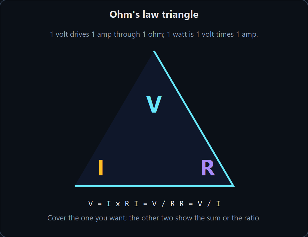
Vector source: docs/assets/diagrams/ohms-law-triangle.svg.

Cover the quantity you want and read what is left: V = I x R, I = V / R, R = V / I. Handy anchors for mental arithmetic: 1 V across 1 k is 1 mA; 5 V across 1 k is 5 mA; 12 V across 1 k is 12 mW; 1 mA through 1 k is 1 V.

Module 19: Series and Parallel Networks

Series and parallel

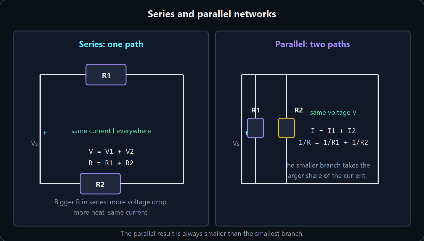
Vector source: docs/assets/diagrams/series-vs-parallel.svg.

The idea. Two parts are in series when they share exactly one node and nothing else joins there, so the same current must pass through both. They are in parallel when both terminals sit on the same two nodes, so the same voltage appears across both. Resistances add in series; conductances (1/R) add in parallel. Capacitors follow the opposite pattern, and so do inductors, because what each element stores decides which quantity is shared.

\(R_{series} = R_1 + R_2 + \dots + R_n, \qquad \frac{1}{R_{parallel}} = \frac{1}{R_1} + \frac{1}{R_2} + \dots\) \(V_{out} = V_{in} \cdot \frac{R_2}{R_1 + R_2}, \qquad I_1 = I_{total} \cdot \frac{R_2}{R_1 + R_2}\)

Worked example. A 5 V source with 0.2 ohm of output resistance feeds three parallel resistors, 100 ohm, 220 ohm and 470 ohm. The parallel value is 59.9 ohm, so the total including the source resistance is 60.1 ohm and the source current is 83.2 mA. The node sits at 4.987 V instead of 5.000 V, and the branch currents are 49.9 mA, 22.7 mA and 10.6 mA: they add up to 83.2 mA, which is Kirchhoff's current law checking the arithmetic. Remove the 100 ohm branch and the parallel value rises to 150 ohm, the node to 4.9934 V and the source current falls to 33.3 mA.

Try it in Bastion. Open examples/voltage_divider.eda.json, then add a second lower-leg resistor and watch both the output voltage fall and the source current rise. Build the three-branch network above in a scratch schematic and click each branch to compare the currents with the numbers.

Go deeper. Wikipedia Series and parallel circuits (CC BY-SA 4.0, link only) https://en.wikipedia.org/wiki/Series_and_parallel_circuits; Electricity for Boys by J. S. Zerbe, Project Gutenberg ebook 22766 (public domain in the USA) https://www.gutenberg.org/ebooks/22766.

Module 20: Power, Energy and Heat

The idea. Power is a rate and energy is an accumulated amount: \(P = V I\) in watts, \(E = P t\) in joules. A component absorbs power when current flows into its positive terminal while it drops voltage, and the sum over a circuit balances, which is the conservation-of-energy check the simulator runs on every solution. Whatever power a converter does not deliver to its load becomes heat in the converter, and that heat is what decides the package, the heatsink and the cost.

\(P = V I = I^2 R = \frac{V^2}{R}, \qquad E = P t, \qquad \eta = \frac{P_{out}}{P_{in}}\) \(V_{rms} = V_{peak} \sqrt{D} \text{ for a PWM square wave}, \qquad T_j = T_a + P \cdot R_{th}\)

Worked example. A 5 V USB pack with 10 Wh usable feeds a 3.3 V rail through an 88 % efficient buck converter. The 3.3 V side draws 60 mA continuously plus 180 mA for 40 ms every 2 s, so the average current is 60 + 180 x (0.04/2) = 63.6 mA, the load power is 210 mW and the pack supplies 238 mW (the missing 29 mW is heat in the converter). Runtime is 10 Wh / 0.238 W = 42 h, and derating for ageing and cut-off gives a practical 35 h. Raise the radio duty to 20 % and the same arithmetic yields 26 h.

Try it in Bastion. Open examples/led_resistor_circuit.eda.json and read the total dissipation in the circuit stats panel; compare it with the source power. Then open examples/bridge_rectifier_power_supply.eda.json and watch the regulator's dissipation rise as you lower the input voltage or raise the load.

Go deeper. Wikipedia Electric power (CC BY-SA 4.0, link only) https://en.wikipedia.org/wiki/Electric_power; The Boy Electrician by A. P. Morgan, Project Gutenberg ebook 63207 (public domain in the USA) https://www.gutenberg.org/ebooks/63207; Steinmetz, Theory and Calculation of Alternating Current Phenomena (1897, public domain) https://archive.org/details/theoryandcalcul04berggoog.

Module 21: Capacitors and RC Time Constants

RC charging curve

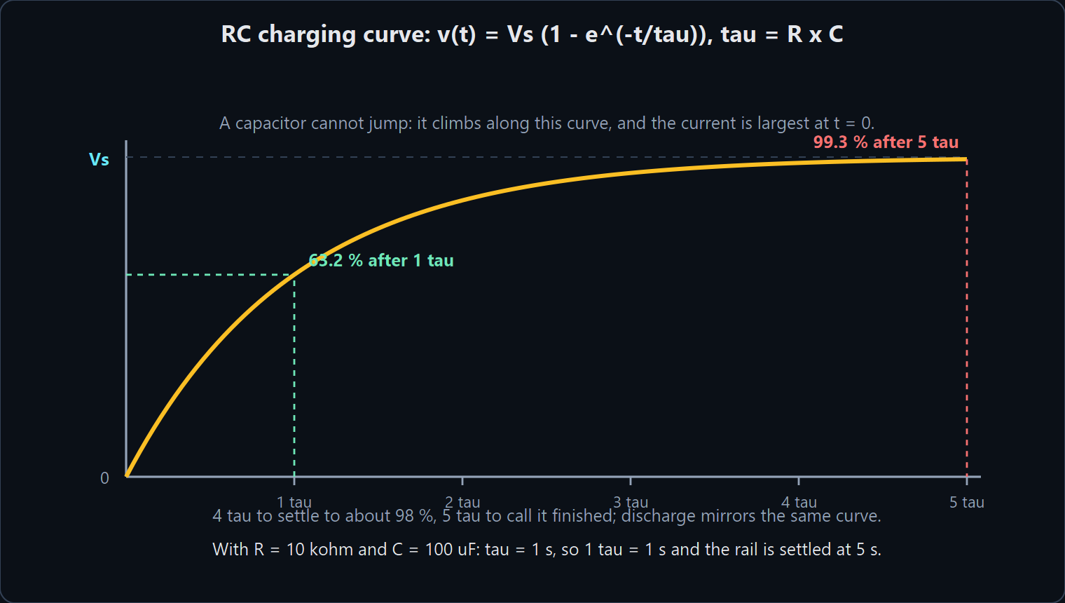
Vector source: docs/assets/diagrams/rc-charging-curve.svg.

The idea. A capacitor stores charge and energy in the electric field between its plates, and its current is proportional to the rate of change of its voltage. That single relation makes the capacitor the element that resists a sudden change of voltage, exactly as the inductor resists a sudden change of current. Charging through a resistor follows an exponential curve whose shape is set by one number, the time constant.

\(Q = C V, \qquad i_C = C \frac{dv}{dt}, \qquad v_C(t) = V_s\left(1 - e^{-t/\tau}\right), \qquad \tau = R C\) \(E = \tfrac{1}{2} C V^2, \qquad X_C = \frac{1}{2 \pi f C}, \qquad t = -\tau \ln\left(1 - \frac{V_t}{V_s}\right)\)

Worked example. A power-on reset charges 100 uF through 10 k toward a comparator that releases at 2.0 V on a 3.3 V rail. The time constant is 1 s, so the release happens at \(t = -1 \ln(1 - 0.606) = 0.93\) s, with an initial current of 3.3 V / 10 k = 330 uA. The rail delivers \(C V^2\) = 1.089 mJ and the capacitor keeps half of it, so 545 uJ is burned in the resistor whatever its value. Later the same 100 uF must cover a 200 mA load pulse lasting 100 us: the charge used is 20 uC, so the rail dips by 0.2 V unless more bulk capacitance or a faster regulator is added.

Try it in Bastion. Open examples/rc_transient_step.eda.json and watch the capacitor voltage climb while the current falls; change R and C separately and watch the curve keep its shape as tau moves. Then open examples/timer_555_monostable.eda.json to see the same exponential used as a timer.

Go deeper. Wikipedia RC circuit (CC BY-SA 4.0, link only) https://en.wikipedia.org/wiki/RC_circuit; Faraday, Experimental Researches in Electricity, volume 1, Project Gutenberg ebook 14986 (public domain in the USA) https://www.gutenberg.org/ebooks/14986.

Module 22: Inductors and the RL Step

The idea. A changing current makes a changing magnetic field, and a changing magnetic field induces a voltage that opposes the change (Faraday's law, with the sign given by Lenz's law). An inductor therefore resists a change of current, stores energy in its field, and generates a voltage spike whenever something tries to interrupt the current suddenly. The time constant of an RL circuit is set by the ratio of inductance to resistance.

\(v_L = L \frac{di}{dt}, \qquad i(t) = \frac{V}{R}\left(1 - e^{-t/\tau}\right), \qquad \tau = \frac{L}{R}\) \(E = \tfrac{1}{2} L I^2, \qquad X_L = 2 \pi f L, \qquad f_0 = \frac{1}{2 \pi \sqrt{L C}}, \qquad Q = \frac{1}{R}\sqrt{\frac{L}{C}}\)

Worked example. A 24 V supply drives a 10 mH, 0.4 ohm solenoid through 20 ohm, with 100 pF of coil capacitance. The steady current is 1.18 A, so the stored energy is \(\tfrac{1}{2} L I^2\) = 6.9 mJ, and the time constant is 10 mH / 20.4 ohm = 0.49 ms, so the coil is energised in about 2.5 ms. The coil's own self-resonance with that 100 pF is at 159 kHz, so any switching must stay well below it. Add a 100 nF snubber across the coil and the pair rings at 5.03 kHz with Q = 0.04: heavily overdamped, which is what a snubber is for.

Try it in Bastion. Open examples/rlc_tank_oscillator.eda.json and watch the ringing decay as you change the series resistance; open examples/hierarchy_rc_filter_chain.eda.json beside it to compare a first-order chain with a second-order ring.

Go deeper. Wikipedia Inductor (CC BY-SA 4.0, link only) https://en.wikipedia.org/wiki/Inductor and LC circuit https://en.wikipedia.org/wiki/LC_circuit; Maxwell, A Treatise on Electricity and Magnetism (1881, public domain) https://archive.org/details/treatiseonelectr01maxwrich.

Module 23: AC Signals, Reactance and Impedance

The idea. A sine averages to zero, so AC quantities need a different description: the RMS value is the DC value that would heat a resistor equally. Reactance is the frequency-dependent opposition of capacitors and inductors, and impedance is the combination of resistance and reactance written as a complex number, so magnitude and phase travel together. Adding reactances as if they were resistances is the classic beginner error.

\(V_{rms} = \frac{V_{peak}}{\sqrt{2}}, \qquad X_C = \frac{1}{2 \pi f C}, \qquad X_L = 2 \pi f L\) \(Z = R + jX, \qquad|Z| = \sqrt{R^2 + X^2}, \qquad \phi = \arctan\left(\frac{X}{R}\right), \qquad P_{real} = V_{rms} I_{rms} \cos \phi\)

Worked example. A 1 uF coupling capacitor feeds a 10 k input impedance. The corner is at 1 / (2 pi x 10 k x 1 uF) = 15.9 Hz, so at 100 Hz the reactance is 1.59 k and the network passes 10/10.13 = 98.7 % with 9 degrees of phase lead; at 10 Hz the reactance rises to 15.9 k and only 53 % of the signal arrives. Reactance tables repay memorising: 100 nF is 31.8 k at 50 Hz, 1.59 k at 1 kHz and 1.59 ohm at 1 MHz, while 10 mH is 3.14 ohm, 62.8 ohm and 62.8 k at the same three frequencies.

Try it in Bastion. Open examples/hierarchy_rc_filter_chain.eda.json and run the AC analysis to see magnitude and phase together. Build a 1 k plus 159 nF series network and check that the two voltages add to 1.41 times the input rather than to the input.

Go deeper. Wikipedia Electrical impedance (CC BY-SA 4.0, link only) https://en.wikipedia.org/wiki/Electrical_impedance; Steinmetz, Theory and Calculation of Alternating Current Phenomena (1897, public domain) https://archive.org/details/theoryandcalcul04berggoog.

Module 24: Filters and Resonance (RC, RL and RLC)

RC low-pass response

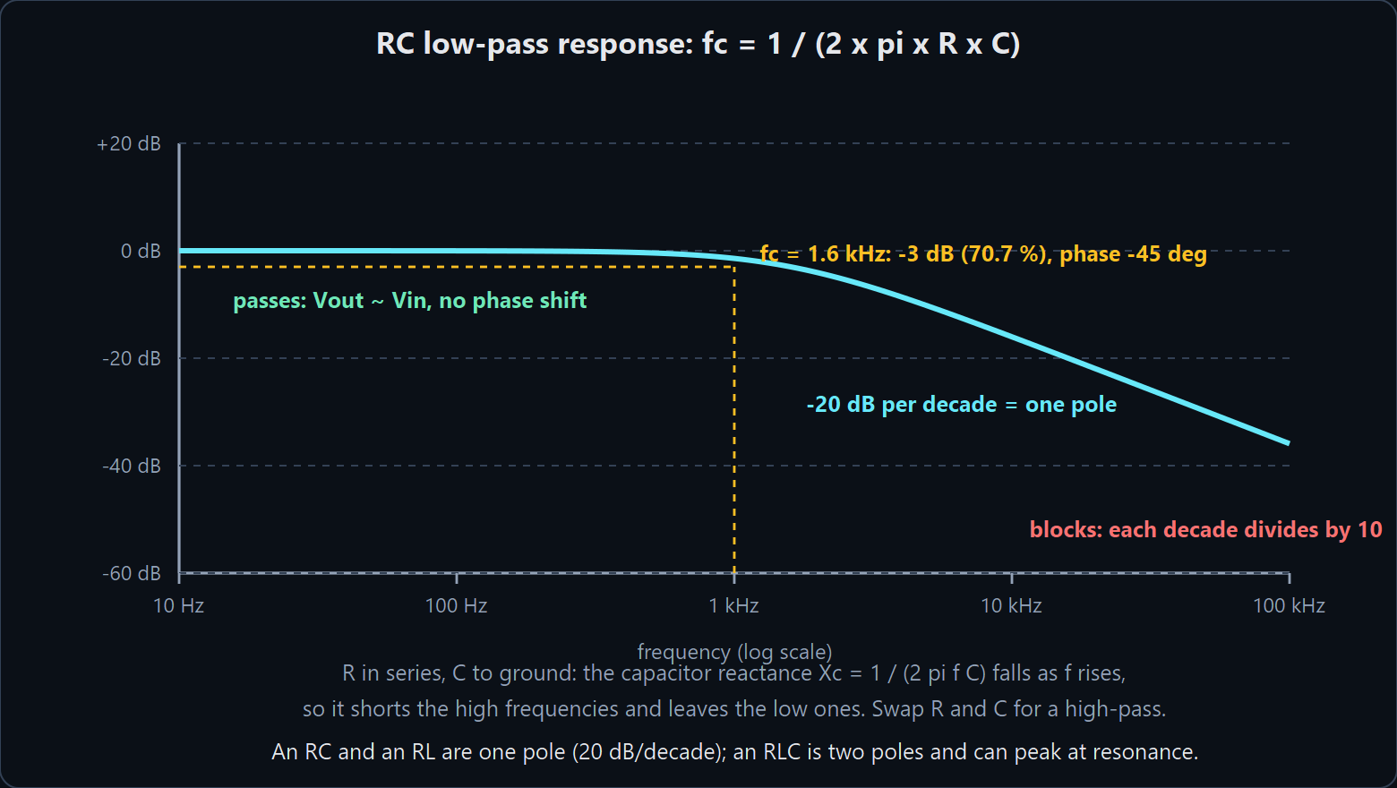
Vector source: docs/assets/diagrams/rc-lowpass-response.svg.

The idea. A resistor with a capacitor or an inductor makes a one-pole filter: flat below the corner, falling at 20 dB per decade above it, with 45 degrees of phase shift at the corner. Two reactances make a second-order filter that rolls off twice as fast, and the same second-order maths gives the sharp peak of resonance. The trade that never goes away is selectivity against settling time: a sharper filter rings longer.

\(f_c = \frac{1}{2 \pi R C} \text{ (RC),} \qquad f_c = \frac{R}{2 \pi L} \text{ (RL)}, \qquad f_0 = \frac{1}{2 \pi \sqrt{L C}}\) \(-3 \text{ dB} = 70.7 \%, \qquad \text{one pole} = -20 \text{ dB/decade}, \qquad Q = \frac{f_0}{BW}\)

Worked example. An anti-alias filter for a 20 kS/s ADC must corner at or below 2 kHz, and the sensor already has 4.7 k of output impedance. Adding a 1 k series resistor makes the total 5.7 k, so \(C = 1/(2 \pi \cdot 2000 \cdot 5700) = 14\) nF, and a 15 nF part puts the corner at 1.86 kHz. At 10 kHz the filter is only 14.6 dB down, so 18.5 % of the interfering signal still arrives; a second identical stage takes that to 29 dB. A 1 k resistor with 100 nF corners at 1.59 kHz, which is the workhorse pair for audio and sensor work, while 10 mH with 100 ohm gives the same corner in the RL form.

Try it in Bastion. Open examples/hierarchy_rc_filter_chain.eda.json and watch the slope and corner move exactly as the formula says; open examples/subcircuit_sallen_key_lpf.eda.json to see a two-pole active filter next to it; open examples/rlc_tank_oscillator.eda.json and watch the phase swing through resonance.

Go deeper. Wikipedia Low-pass filter (CC BY-SA 4.0, link only) https://en.wikipedia.org/wiki/Low-pass_filter, RC circuit https://en.wikipedia.org/wiki/RC_circuit and RLC circuit https://en.wikipedia.org/wiki/RLC_circuit; Steinmetz, Theory and Calculation of Alternating Current Phenomena (1897, public domain) https://archive.org/details/theoryandcalcul04berggoog.

Module 25: Diodes and Rectifiers

Half-wave versus bridge rectifier

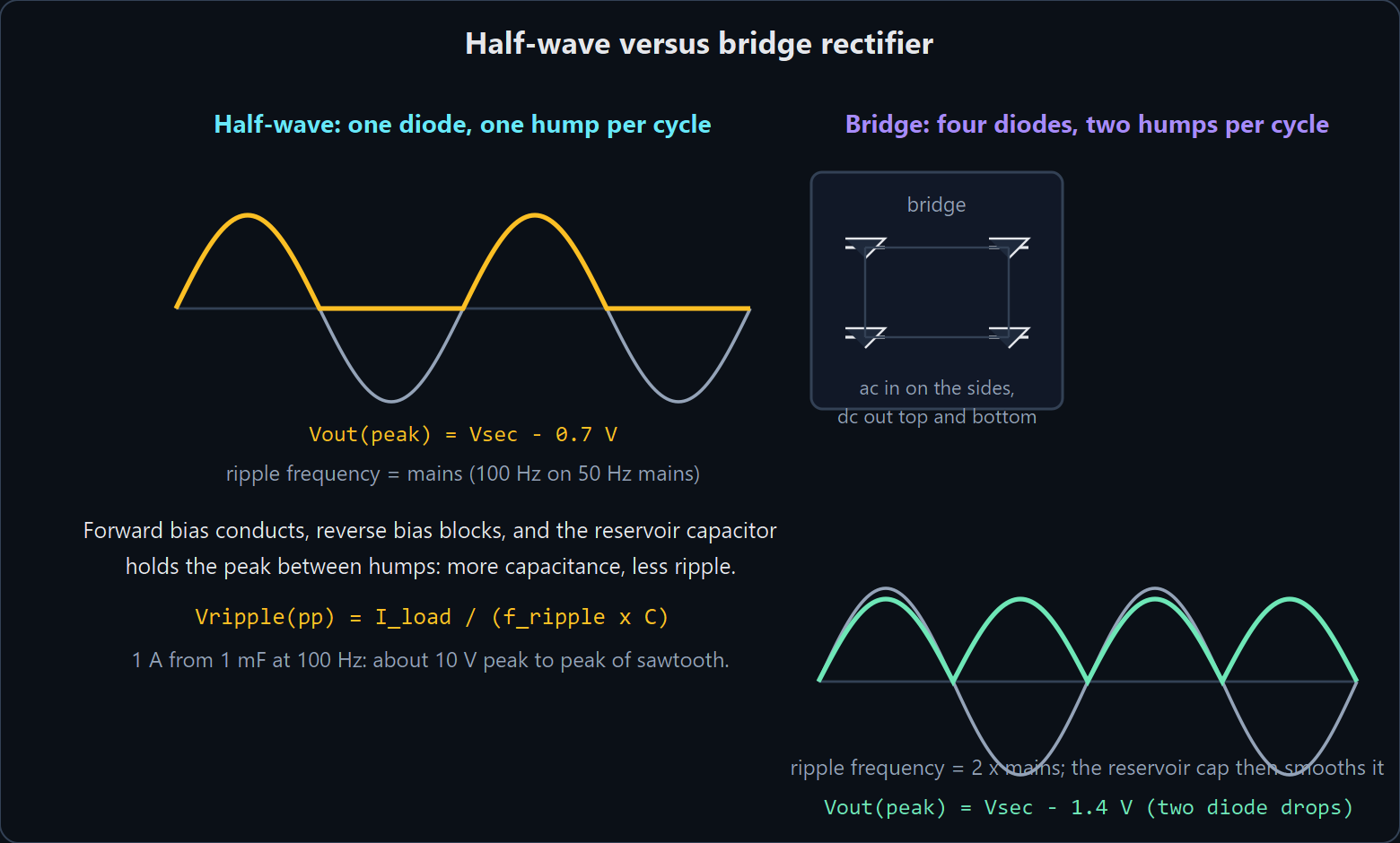
Vector source: docs/assets/diagrams/rectifiers-half-wave-vs-bridge.svg.

The idea. A p-n junction conducts when forward biased and blocks when reverse biased, with a current that rises exponentially at about 60 mV per decade at room temperature. Rectifiers exploit that to turn AC into DC: one diode gives one hump per cycle, a bridge gives two, and a reservoir capacitor fills the gaps between humps. The peak current through the diodes is far larger than the DC load current because the capacitor only accepts charge near the peak.

\(I_D = I_S \left(e^{V_D / n V_T} - 1\right), \qquad V_T = 26 \text{ mV at } 300 \text{ K}\) \(V_{ripple(pp)} = \frac{I_{load}}{f_{ripple} C}, \qquad V_{out(peak)} = V_{peak} - 0.7 \text{ V (one diode)} - 1.4 \text{ V (bridge)}\)

Worked example. A 12 V RMS transformer bridge feeds a 4700 uF reservoir into a 1 A load. The secondary peak is 17.0 V and two diode drops bring the capacitor to 15.4 V; the ripple is 1 A / (100 Hz x 4700 uF) = 2.1 V peak to peak, so the rail averages 14.3 V and never falls below 13.3 V. The peak repetitive diode current is roughly 4 A, the capacitor's ripple current is about 1.4 A RMS (which is what decides its life) and the peak inverse voltage is only the transformer's 17 V, so a 1000 V 1N4007 is pure headroom. Halving the capacitance doubles the ripple and lowers the average output.

Try it in Bastion. Open examples/diode_rectifier_limiter.eda.json and watch the clipper flatten one half of the waveform, then reverse the diode; open examples/bridge_rectifier_power_supply.eda.json and probe the secondary, the rectified node and the smoothed rail together.

Go deeper. Wikipedia Rectifier (CC BY-SA 4.0, link only) https://en.wikipedia.org/wiki/Rectifier, Diode bridge https://en.wikipedia.org/wiki/Diode_bridge and Diode https://en.wikipedia.org/wiki/Diode; The Boy Electrician (Project Gutenberg ebook 63207, public domain in the USA) https://www.gutenberg.org/ebooks/63207.

Module 26: Transistors (BJT): Switches and Amplifiers

NPN transistor as a switch

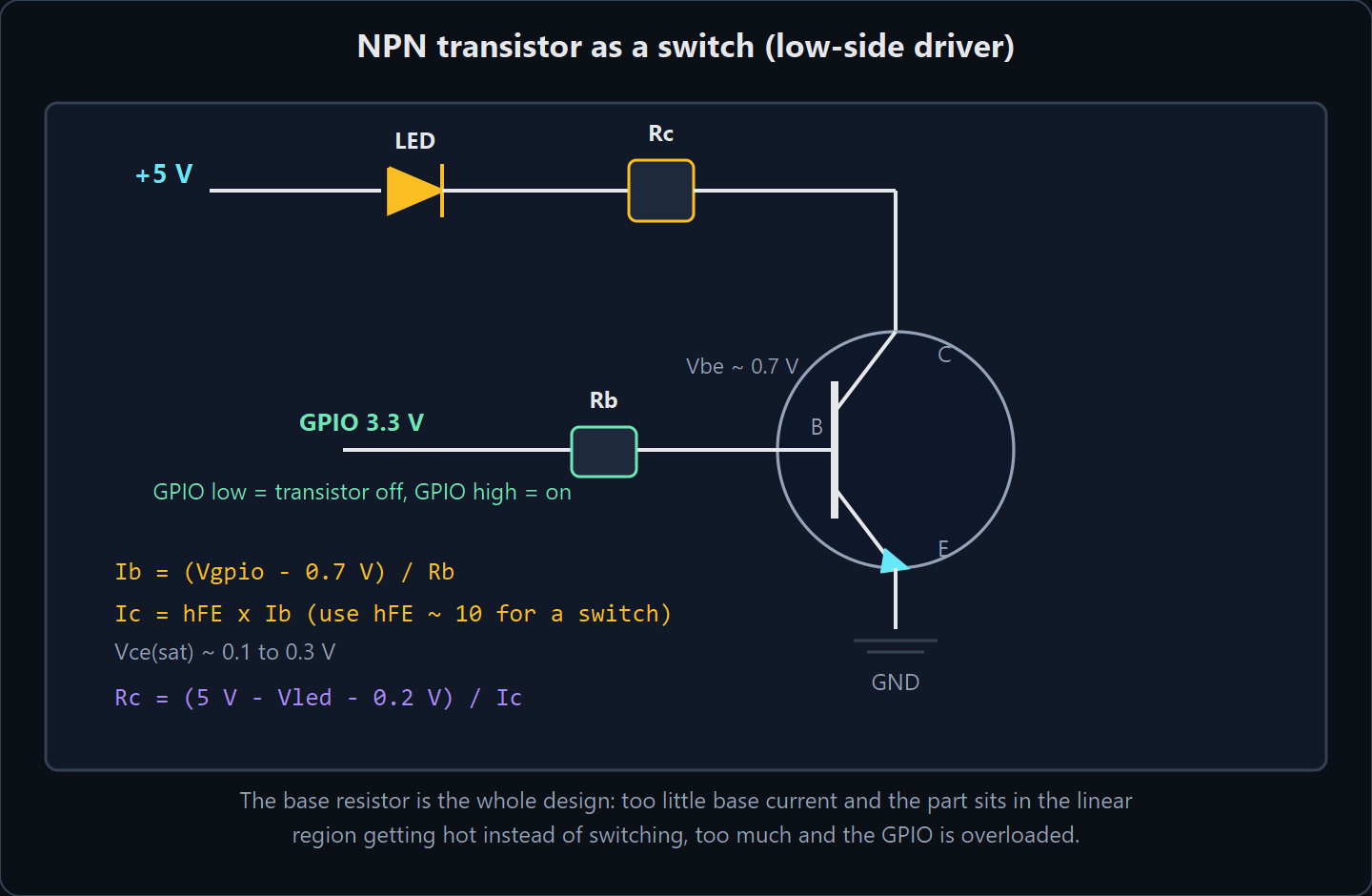
Vector source: docs/assets/diagrams/bjt-switch.svg.

The idea. A bipolar transistor is two junctions sharing a thin base, so a small base current controls a much larger collector current: \(I_C = \beta I_B\). Beta is not a design number - it varies threefold between parts and rises with temperature - so a switch is designed with a forced beta of about 10 to guarantee saturation, and an amplifier is designed so that the bias depends on resistors rather than on beta. A switch lives in cutoff and saturation; an amplifier lives in the active region and pays for its linearity with continuous dissipation.

\(I_C = \beta I_B, \qquad I_E = I_C + I_B, \qquad V_{BE} \approx 0.7 \text{ V}, \qquad V_{CE(sat)} \approx 0.1 \dots 0.3 \text{ V}\) \(I_B = \frac{I_C}{10} \text{ (forced beta for a switch)}, \qquad R_B = \frac{V_{drive} - V_{BE}}{I_B}, \qquad g_m = \frac{I_C}{26 \text{ mV}}, \qquad A_v = -g_m R_C\)

Worked example. An NPN transistor drives three white LEDs (9.3 V of forward drop) at 92 mA from a 12 V rail, controlled by a 3.3 V GPIO. The collector resistor is (12 - 9.3 - 0.2)/0.1 = 25 ohm, so 27 ohm gives 92 mA. With a forced beta of 10 the base current is 9.2 mA and the base resistor is (3.3 - 0.9)/9.2 mA = 260 ohm, so 270 ohm. The transistor dissipates only 0.2 V x 92 mA = 18 mW, the base resistor 21 mW, and the LED string 856 mW - the heat is in the LEDs, not the switch. The GPIO sources 8.9 mA against a 20 mA limit, leaving 11 mA of the pin's budget for everything else.

Try it in Bastion. Open examples/bjt_audio_amplifier.eda.json and watch the collector sit at its bias point, then change the base divider and watch the quiescent current move; open examples/motor_driver_l293d.eda.json to see the same saturation arithmetic applied twice per motor terminal inside a bipolar bridge.

Go deeper. Wikipedia Bipolar junction transistor (CC BY-SA 4.0, link only) https://en.wikipedia.org/wiki/Bipolar_junction_transistor and Common emitter https://en.wikipedia.org/wiki/Common_emitter; The Boy Electrician (Project Gutenberg ebook 63207, public domain in the USA) https://www.gutenberg.org/ebooks/63207.

Module 27: MOSFETs as Switches

The idea. A MOSFET is switched by an electric field across an insulated gate, so it draws no steady gate current and its on-resistance is what decides the loss. The threshold voltage is where conduction starts, not where the part is useful: read the Rds(on) figure and the gate voltage it is quoted at, and remember that Rds(on) rises by 50 % to 80 % from 25 degC to 100 degC. An N-channel device is easiest on the low side, where its source is at ground and a logic-level gate voltage is plenty.

\(P_{cond} = I_D^2 R_{DS(on)}(T), \qquad T_j = T_a + P_{cond} R_{th(j-a)}\) \(t_{switch} \approx \frac{Q_g}{I_{gate}}, \qquad I_{gate} = \frac{V_{drive} - V_{th}}{R_{gate}}\)

Worked example. A 12 V, 1 A LED strip is switched by a logic-level N-channel MOSFET from a 3.3 V pin through a 100 ohm gate resistor. The part must have Rds(on) well under 0.1 ohm at 3.3 V gate drive, say 0.05 ohm cold and 0.08 ohm hot: the conduction loss is 50 mW cold and 80 mW hot, and with 50 degC/W junction-to-ambient that is a 4 degC rise, so no heatsink is needed. The gate charge of 10 nC driven at (3.3 - 2)/100 = 13 mA switches in about 0.8 us, fast enough that switching loss is negligible below 10 kHz. At 5 A the same part would dissipate 2 W and need a DPAK on copper or two devices in parallel.

Try it in Bastion. Open examples/mosfet_led_switch.eda.json and watch the drain fall to millivolts when the gate is high; drop the gate drive from 5 V to 3.3 V and read the on-state drain-source voltage to see Rds(on) change; open examples/motor_driver_l293d.eda.json to compare its bipolar saturation drops with the MOSFET switch.

Go deeper. Wikipedia MOSFET (CC BY-SA 4.0, link only) https://en.wikipedia.org/wiki/MOSFET and Power MOSFET https://en.wikipedia.org/wiki/Power_MOSFET; The Boy Electrician (Project Gutenberg ebook 63207, public domain in the USA) https://www.gutenberg.org/ebooks/63207.

Module 28: Op-Amps: Inverting and Non-Inverting

Op-amp gain configurations

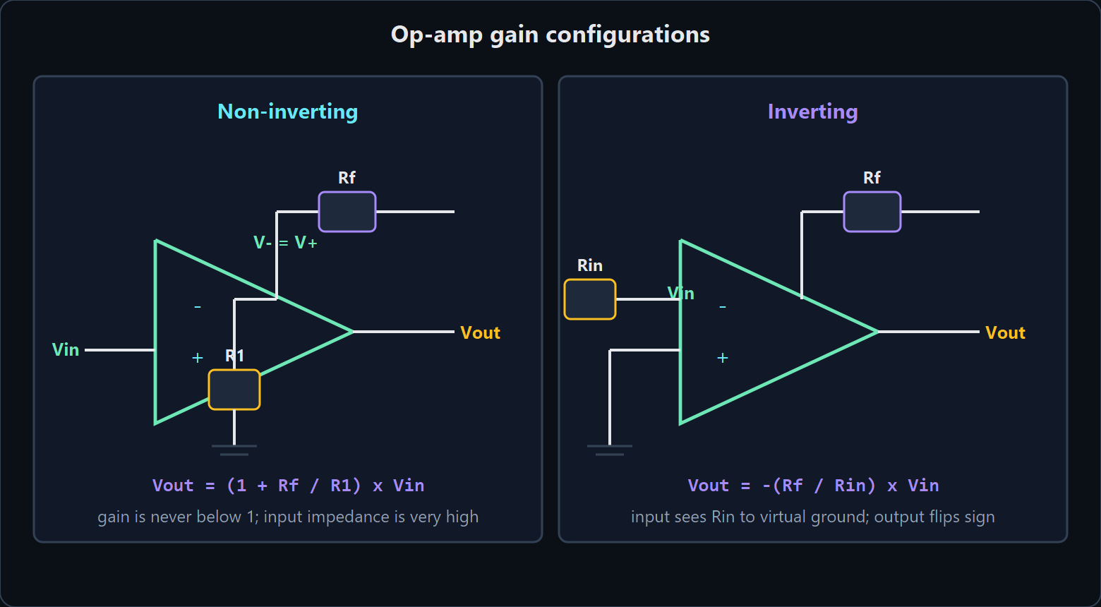
Vector source: docs/assets/diagrams/opamp-noninverting.svg.

The idea. An op-amp has enormous open-loop gain, so with negative feedback it needs only microvolts between its inputs to produce any sane output. That gives the two golden rules: the inputs sit at the same voltage (virtual short) and they draw no current. Both hold only while the output is not saturated. The feedback network then decides everything: the non-inverting form never attenuates, the inverting form inverts and presents Rin as its input impedance, and the input offset voltage is amplified by exactly the same gain as the signal.

\(V_{out} = \left(1 + \frac{R_f}{R_1}\right) V_{in} \text{ (non-inverting)}, \qquad V_{out} = -\frac{R_f}{R_{in}} V_{in} \text{ (inverting)}\) \(GBW = \text{gain} \times \text{bandwidth}, \qquad \text{slew rate} \geq 2 \pi f V_{peak}\)

Worked example. A 5 mV strain-gauge signal must reach a 3.3 V ADC, so the gain needed is about 200. Done in one non-inverting stage with Rf = 200 k and R1 = 1 k, a 3 mV input offset becomes 600 mV of output error, which is 300 counts on a 12-bit converter. Split into two stages of 20 and 10 and the same 3 mV (6 mV worst case across two parts) becomes 60 mV before the second stage adds its own 10 mV. A 1 MHz gain-bandwidth part in a gain of 20 gives 50 kHz of bandwidth, comfortably above a 100 Hz load-cell signal, and 1 % resistors give about 2 % of gain error which calibration removes.

Try it in Bastion. Open examples/opamp_noninverting_amp.eda.json and confirm that V+ equals V- in the results, then change Rf and watch the gain follow 1 + Rf/R1; wire the same parts as an inverting amplifier in a scratch schematic and watch the output invert and the input impedance become Rin.

Go deeper. Wikipedia Operational amplifier (CC BY-SA 4.0, link only) https://en.wikipedia.org/wiki/Operational_amplifier and Negative-feedback amplifier https://en.wikipedia.org/wiki/Negative-feedback_amplifier; Steinmetz, Theory and Calculation of Alternating Current Phenomena (1897, public domain) https://archive.org/details/theoryandcalcul04berggoog.

Module 29: Logic Gates and Combinational Logic

The idea. Every gate is a truth table, and every truth table has a mechanical realisation: one AND per row of ones and an OR to collect them. NAND and NOR are universal - either one alone builds NOT, AND and OR

which is why CMOS libraries are full of NANDs. The engineering work is in the corners: unused inputs must never float, families differ in thresholds and drive strength, and a combinational output that glitches for a few nanoseconds must never be wired straight into a clock, reset or interrupt pin.

\(Y = \overline{A \cdot B} \text{ (NAND)}, \qquad \overline{A \cdot B} = \overline{A} + \overline{B} \text{ (De Morgan)}, \qquad P_{dyn} = C_L V_{DD}^2 f\) \(t_{ripple} = N \cdot t_{bit} \text{ (ripple-carry adder)}\)

Worked example. A 4-bit comparator built from 74HC parts needs about three gate levels for the top bit and another level per lower bit: roughly 15 ns per level gives 45 ns for the first comparison and 90 ns for the worst case, so a registered design can run at up to about 10 MHz. The same reasoning sizes a ripple-carry adder: four bits at about 12 ns of carry prop each is 48 ns, which is why wider adders use carry-look-ahead or parallel-prefix structures that trade gates for depth. Note the second half of the lesson: a design that is fast enough on paper still fails if a two-input change produces a glitch that reaches an edge-sensitive pin.

Try it in Bastion. Open examples/digital_half_adder.eda.json and click the sum and carry nets for all four input combinations; open examples/mixed_signal_logic.eda.json to watch a gate driven from an analogue node cross its switching threshold.

Go deeper. Wikipedia Logic gate (CC BY-SA 4.0, link only) https://en.wikipedia.org/wiki/Logic_gate, Boolean algebra https://en.wikipedia.org/wiki/Boolean_algebra and Adder (electronics) https://en.wikipedia.org/wiki/Adder_(electronics); How it Works by Archibald Williams, Project Gutenberg ebook 28553 (public domain in the USA) https://www.gutenberg.org/ebooks/28553.

Module 30: PWM: Duty Cycle, Motors and Relays

PWM duty cycle

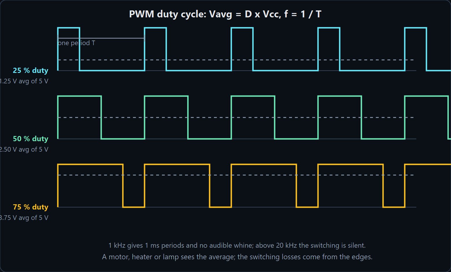
Vector source: docs/assets/diagrams/pwm-duty-cycle.svg.

The idea. PWM switches a supply on and off fast enough that the load responds to the average. Three of its numbers matter for different reasons: the average is what a meter or a filtered PWM shows, the RMS value is what heats a resistor, and the peak is what a semiconductor must survive. A low-pass filter turns the pulses into a quasi-DC level, and the price of a clean level is settling time. Inductive loads need their freewheel path whatever the duty cycle, because the spike is generated by the current at every edge.

\(V_{avg} = D V_{cc}, \qquad V_{rms} = V_{cc}\sqrt{D}, \qquad P = D \frac{V^2}{R}\) \(V_{ripple} \approx \frac{V_{cc} D (1 - D) T}{R C} \text{ (RC filter)}, \qquad \Delta I = \frac{V D (1 - D) T}{L} \text{ (inductive load)}\)

Worked example. A 12 V relay or solenoid coil of 0.3 H and 120 ohm pulls in at 100 % duty and then holds at 30 % duty: the average current falls from 100 mA to 30 mA, saving 0.84 W, while the freewheel diode still absorbs the kick at every edge. At 1 kHz the current ripple is 12 x 0.3 x 0.7 x 1 ms / 0.3 H = 8.4 mA, so the coil current is a smooth 30 mA. As a DAC, 5 V PWM at 20 kHz through 1 k and 10 uF has 6.25 mV of ripple - a third of an 8-bit step - but needs 50 ms to settle, which is the whole trade-off in one number.

Try it in Bastion. Put a PWM source through an RC filter in a scratch schematic and watch the ripple collapse as the corner frequency falls; open examples/motor_driver_l293d.eda.json and raise the PWM frequency to see the motor current smooth out; open examples/subcircuit_555_astable.eda.json to see the timing side of the same pulsing.

Go deeper. Wikipedia Pulse-width modulation (CC BY-SA 4.0, link only) https://en.wikipedia.org/wiki/Pulse-width_modulation and Flyback diode https://en.wikipedia.org/wiki/Flyback_diode; The Boy Electrician (Project Gutenberg ebook 63207, public domain in the USA) https://www.gutenberg.org/ebooks/63207.

Module 31: Grounding, Noise and Decoupling

The idea. Ground on a schematic is one node; on a board it is copper with resistance and inductance, so any current shared between two circuits appears as a voltage to the quieter one. At DC the return current takes the path of least resistance; at high frequency it takes the path of least inductance, directly under the signal trace. Decoupling capacitors are local charge reservoirs whose value matters less than their placement, because the dip during a fast edge is set by the loop inductance, not by the missing charge. Capacitance answers "how much charge is available"; inductance answers "how fast can it arrive".

\(v = L \frac{di}{dt}, \qquad Z_{target} = \frac{V_{ripple(allowable)}}{I_{transient}}, \qquad X_C = \frac{1}{2 \pi f C}\)

Worked example. An MCU draws 20 mA on average but 100 mA for 2 ns at each internal clock edge, needing 200 pC - only 0.06 % of the charge held by a 100 nF capacitor at 3.3 V, so capacitance is never the problem. With the capacitor 10 mm away (about 10 nH of loop inductance) the dip is 10 nH x 0.1 A / 2 ns = 0.5 V, which is 15 % of the rail and enough to reset the chip. With the part 1 mm away (1 nH) the dip is 50 mV. Slowing the edge to 10 ns with a series resistor or a lower drive strength brings it to 10 mV.

Try it in Bastion. Open examples/rp2040_blinky.eda.json and watch the supply node hold steady while the GPIO switches, then delete the decoupling capacitance in a scratch circuit and watch the spikes appear; open examples/mcu_i2c_sensor_workbench.eda.json and look at the bus and its pull-ups.

Go deeper. Wikipedia Ground (electricity) (CC BY-SA 4.0, link only) https://en.wikipedia.org/wiki/Ground_(electricity), Ground loop (electricity) https://en.wikipedia.org/wiki/Ground_loop_(electricity) and Decoupling capacitor https://en.wikipedia.org/wiki/Decoupling_capacitor; The Standard Electrical Dictionary, Project Gutenberg ebook 26535 (public domain in the USA) https://www.gutenberg.org/ebooks/26535.

Study material: 58 lessons

Every lesson now goes beyond the short card (governing law, key equations, core concept, rule of thumb): it has several headed sections that explain the idea step by step, a worked example with numbers, a list of common mistakes, a Try it in Bastion list of things to build and measure in the simulator, self-check questions with answers, and links to related lessons. The material is stored as embedded JSON in src/Bastion.Core/Education/Content/ (one array of lessons per file); a lesson whose Id already exists in the built-in cards only adds its study material, any other lesson is added whole. A synchronised short card from the curriculum repository never erases the study material.

Reading times are computed by the Academy from the lesson text at 200 words per minute, and the word count covers the long-form study material (sections, worked example, common mistakes and the bench exercises). The lessons marked with a four-figure count were expanded in this pass; before it, every one of them was about 400 words.

To add a lesson, append an object with the same fields as the existing ones (Id, Title, Category, GoverningLaw, KeyFormulas, Summary, DeepDive, EngineeringRuleOfThumb, AssociatedComponentIds, Keywords, Level, Sections, WorkedExample, CommonMistakes, TryInBastion, Quiz, RelatedLessonIds) to one of the files; Phase91AcademyAndInterfaceTests checks the structure (at least three sections, a worked example, two questions, links that resolve).

Sources, licences and how to reuse this page

Everything on this page is written for Bastion. The explanations, the worked examples and the diagrams are our own prose and our own drawings; no text has been copied from any source, and no diagram has been traced from another work. The links below are credits and pointers for further study, and every one of them was checked live when this page was last edited (November 2026). Every listed source permits commercial reuse (public domain, CC0 or CC BY), so the material may be built on by anyone; nothing is reproduced from it.

Commercially reusable (public domain, CC BY or CC BY-SA when linked)

A word of caution for anyone reusing material from the web: licences change, and a reference that was free to reuse years ago may carry a non-commercial licence today - that is what happened to the two physics textbooks that older notes here linked. Check the licence on the page you are actually copying from, and prefer the public-domain texts in the table above when you need something you can print, modify or sell.

Attribution policy

Only commercially reusable material is credited or linked on this page: public domain, CC0, CC BY, or CC BY-SA where the source is linked as a pointer and its text is never copied. Non-commercial material (courseware under a non-commercial licence and the like) is not credited, listed or linked here at all. The eighteen modules that open the page name their references in an Open-Source Attribution line, which is kept to the same rule.

Accessing Lessons Inside Bastion Circuit Designer

Bastion provides 4 interconnected access points for educational physics and electricity theory:

Interactive Canvas Hover HUD Tooltips:

Hover your mouse cursor over any component or net wire on the schematic canvas.
Bastion displays a rich, translucent educational tooltip showing the component's name, governing physical law, formula, physical summary, and engineering rule of thumb.
Can be toggled in View > Toggle Physics Canvas Tooltips.

Properties Inspector Card (Right Sidebar):

Select any component on the canvas.
The right sidebar displays the Physics & Electrical Theory card containing the governing equation, concept summary, rule of thumb, and a Read Full Physics Lesson... button.

Dedicated Physics & Electricity Academy Window (Ctrl+Shift+L):

Open via Help > Physics & Electricity Lessons... or Tools > Physics & Electricity Academy... or pressing Ctrl+Shift+L.
Search across topics or filter by category.
View deep-dive physics, equation blocks, and open-source attributions.
Click Place Associated Component to immediately instantiate related components onto your active canvas!

Multimodal AI Co-Pilot Pair Programming:

Ask the AI Co-Pilot (AI Co-Pilot panel) any question about voltage, current, Ohm's law, op-amps, or circuit theory.
The AI cites the authoritative open-source references, explains governing equations, and automatically opens the Academy topic for you!